In the era of exascale computing, the bottleneck is no longer just calculation speed, but data movement and energy consumption. Mixed-precision algorithms offer a compelling solution by combining the speed of low-precision arithmetic with the accuracy of high-precision formats.
1. The Anatomy of Floating-Point Numbers
To understand mixed-precision, we must first rigorously define how computers represent real numbers. According to the IEEE 754 standard, a floating-point number is represented as:
$$ x = (-1)^s \times M \times 2^{E - B} $$Where $s$ is the sign bit, $M$ is the mantissa (significand), $E$ is the exponent, and $B$ is the bias. The trade-off between precision and range is determined by how we allocate bits to the Exponent and the Fraction (Mantissa).
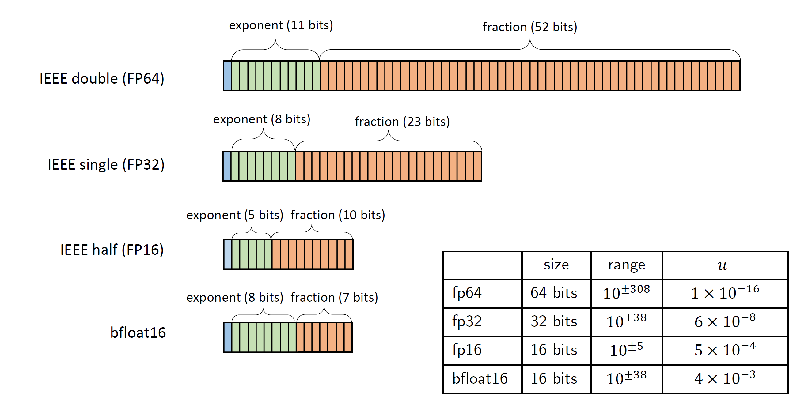
As illustrated in Figure 1, different formats allocate these bits differently:
- FP64 (Double Precision): Standard for scientific simulation. High precision (~16 decimal digits).
- FP32 (Single Precision): Standard for legacy graphics and general computing.
- FP16 / BF16 (Half Precision): Reduced exponent or fraction bits. Significantly faster and uses less memory, but prone to overflow (range issues) or rounding errors (precision issues).
2. Mixed-Precision Iterative Refinement
The core idea of mixed-precision algorithms is not simply "using lower precision," but strategically combining precisions to maintain accuracy. A classic example in Numerical Linear Algebra is Iterative Refinement for solving linear systems $Ax=b$.
The algorithm generally follows these steps:
- Factorization (Low Precision): Decompose the matrix $A$ (e.g., LU decomposition) in low precision ($u_{low}$) to obtain approximate factors $L, U$. This is the most computationally expensive step but is accelerated by low precision (e.g., FP16). $$ P A \approx L U $$
- Compute Residual (High Precision): Calculate the residual $r$ in high precision ($u_{high}$) using the current solution approximation $x_k$. $$ r_k = b - A x_k $$
- Solve Correction (Low Precision): Solve for the correction term $d_k$ using the low-precision factors. $$ L U d_k = r_k $$
- Update Solution (High Precision): Update the solution vector. $$ x_{k+1} = x_k + d_k $$
"By computing the expensive $O(n^3)$ factorization in low precision and the cheaper $O(n^2)$ matrix-vector products in high precision, we achieve the best of both worlds."
3. Error Analysis and Convergence
The convergence of this method depends heavily on the condition number of the matrix, $\kappa(A)$, and the unit roundoff of the low-precision format, $u_{low}$. A sufficient condition for convergence is generally:
$$ \kappa(A) \cdot u_{low} < 1 $$This inequality highlights a critical constraint: if the matrix is too ill-conditioned, or if the low precision is too coarse (e.g., FP16 has a very small dynamic range), the algorithm may fail to converge. This necessitates the use of more robust scaling techniques or alternative formats like BFloat16.
4. Conclusion
Mixed-precision algorithms represent a paradigm shift in scientific computing. They allow us to leverage the hardware accelerators (like Tensor Cores) originally designed for Deep Learning to accelerate traditional scientific simulations, achieving optimal trade-offs between accuracy, performance, and energy efficiency.